Intelligent Robotic Arm: Vision-Based Control and EMG-Driven Gesture Recognition

Abstract

This report documents the design decisions, implementation challenges, and experimental results encountered while building a MediaPipe-based hand tracking pipeline to control a tendon-driven robotic hand. We focus on two tightly coupled problems: robust thumb angle estimation and the trade-off between responsiveness and stability introduced by temporal smoothing.

We describe the geometric approaches explored for thumb angle computation, the smoothing methods implemented, and an offline evaluation framework based on logged trajectories. Experimental results show that while smoothing is effective for non-thumb fingers, thumb performance is fundamentally limited by geometric ambiguity rather than temporal noise.

A second, independent part of the project develops an EMG-driven gesture recognition pipeline. It covers synthetic signal generation for pipeline validation, configuration-driven preprocessing, and three modelling families evaluated on that synthetic data: recurrent networks (GRU and LSTM), a lightweight convolutional network operating on log-mel spectrograms, and a classical machine-learning baseline.

System Overview

Runtime pipeline

1. Vision: Webcam input processed using MediaPipe Hands to extract 2D hand landmarks.
2. Geometry: Landmark positions are used to estimate a palm reference plane and per-finger flexion angles.
3. Smoothing: Temporal filtering is applied to $[\theta_{\text{thumb}},\ \theta_{\text{index}},\ \theta_{\text{middle}},\ \theta_{\text{ring}},\ \theta_{\text{pinky}},\ \text{roll},\ \text{pitch}]$.
4. Calibration and mapping: Open and fist poses define a linear mapping from angles to servo targets.
5. Actuation: Quantized servo commands are transmitted over serial once calibration is completed.

Serial communication and quantization

After smoothing and calibration-based mapping, each servo target is quantized to one-degree increments before transmission. Commands are sent over a serial link in a compact formatted packet containing all finger and wrist targets.

Quantization reduces small frame-to-frame fluctuations that would otherwise cause unnecessary micro-movements of the servos. This improves practical control stability and reduces visible actuator chatter.

Mathematical Formulation

Palm plane estimation

Let the selected palm landmarks be

where each point corresponds to the wrist or an MCP joint. The centroid is

The covariance matrix is

The palm normal is given by the eigenvector corresponding to the smallest eigenvalue of $C$.

Finger flexion angle

For a finger defined by landmarks $a$ and $b$, let $v = b - a$ and let $n$ be the palm normal. The flexion angle is computed as

and clamped to $[0^{\circ}, 90^{\circ}]$.

Servo mapping

EMA smoothing

Calibration and Safety Mechanisms

User-guided calibration

The system uses two manually captured reference poses:

• an open pose, representing the fully extended hand,
• a fist pose, representing the closed hand.

These define the valid operating range for each finger and are stored for later reuse.

Control gating

Servo commands are not transmitted until calibration has been completed. This prevents accidental motion caused by default mappings, invalid pose ranges, or startup noise. From an engineering perspective, this gating mechanism acts as a safety layer between perception and actuation.

Thumb Angle Estimation

Why the thumb is fundamentally different

For the index, middle, ring, and pinky fingers, flexion can be approximated by the angle between a finger segment and a palm reference plane. The thumb differs in several key aspects:

1. The thumb combines flexion/extension and abduction/adduction in a single observed motion.
2. Its base joint is offset relative to the palm and rotates about a different anatomical axis.
3. Thumb landmarks are more sensitive to occlusions, perspective effects, and wrist rotation.

As a result, a single scalar angle is an imperfect representation of thumb motion.

Palm normal estimation

We estimate a palm normal using PCA on a subset of stable landmarks (wrist and MCP joints). This provides a robust reference for most fingers, but introduces several limitations:

• The estimated normal can drift under wrist rotation or partial occlusion.
• The normal direction is sign-ambiguous and must be flipped heuristically.
• Errors in the palm normal directly propagate to all angle estimates that depend on it.

Thumb angle strategies explored

Direct palm-normal method. We initially treated the thumb identically to other fingers, computing its angle relative to the palm normal. This approach proved highly sensitive to wrist orientation and resulted in frequent sign flips and large angle discontinuities.

Offset plane method (implemented). The final implemented method modifies the palm reference plane by tilting it toward the thumb’s dominant direction of motion and offsetting its centroid toward the thumb base. Thumb flexion is computed as the angle between the thumb direction vector and this adjusted plane, followed by range clamping.

Thumb-local reference plane (tested). We also implemented a thumb-local reference plane defined using the wrist, thumb base, and index MCP landmarks. In practice, this approach produced increased lag and jitter compared to the offset plane method.

A likely cause is that the thumb-local plane relies on a smaller set of landmarks that are themselves highly mobile. As a result, the reference plane becomes non-stationary, amplifying landmark noise and introducing rapid orientation changes. While this hypothesis is consistent with observed behavior, a more controlled evaluation with raw landmark logging would be required to confirm it.

Offset-plane thumb model

The palm reference plane is modified by tilting its normal toward the thumb motion direction and shifting its centroid toward the thumb base. This produces a thumb-specific reference plane that is less tightly coupled to the central palm geometry.

In practice, this improves continuity compared to the direct palm-normal method, although it remains sensitive to wrist rotation and landmark instability. The method should therefore be viewed as a geometric heuristic rather than a full anatomical model.

Observed practical issues

Across all thumb angle formulations, we observed:

• Oscillations near mid-range thumb bends.
• Sudden spikes caused by single-frame landmark inconsistencies.
• Strong coupling between thumb angle and wrist rotation.

Temporal Smoothing

We evaluated three smoothing configurations:

1. No smoothing: maximum responsiveness with significant temporal noise.
2. Exponential Moving Average (EMA): fixed low-pass filtering.
3. One Euro Filter: adaptive cutoff frequency based on signal velocity.

Smoothing was applied uniformly across all fingers and wrist signals.

Experimental Evaluation

Logged data

Each experimental run produces two CSV files:

• raw.csv: time-stamped detected angles used at runtime.
• quant.csv: corresponding quantized servo commands.

The logs store post-geometry, post-smoothing angles rather than raw landmarks.

Metrics

For each finger and each run, we computed:

• Jitter: standard deviation during an initial hold-still window.
• RMSE: root mean squared error between detected and commanded trajectories.
• High-frequency ratio: fraction of spectral energy above $3\ \text{Hz}$.
• Fast and slow error: mean absolute error during fast and slow commanded segments.

Fast and slow segments are identified from the commanded trajectory.

Results

Quantitative results

Table 1: Thumb performance metrics (normalized units).

Table 2: Index finger performance metrics (normalized units).

Thumb: per-run trajectories

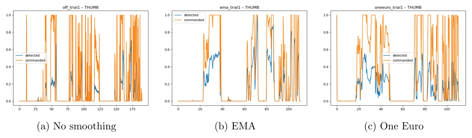
Interpretation. The thumb trajectories show large deviations between detected and commanded signals across all configurations. EMA produces the smoothest trajectory but still exhibits substantial lag during fast motion. No smoothing results in sharp discontinuities, while One Euro filtering reduces high-frequency noise but introduces additional delay and overshoot. These effects are consistent with thumb instability being dominated by geometric factors rather than temporal noise alone.

Thumb: error distributions

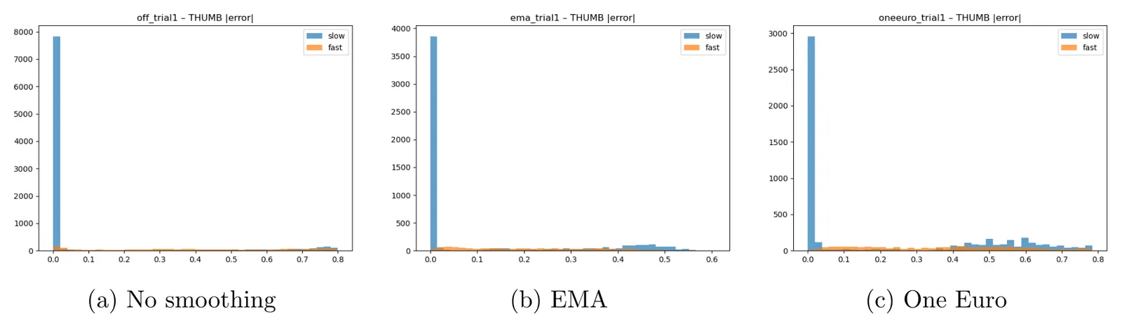
Interpretation. Fast-segment errors are substantially larger than slow-segment errors for all smoothing configurations, confirming that rapid thumb motions exacerbate geometric instability. EMA reduces the overall error magnitude, whereas no smoothing produces extreme outliers during fast motion.

Index: per-run trajectories

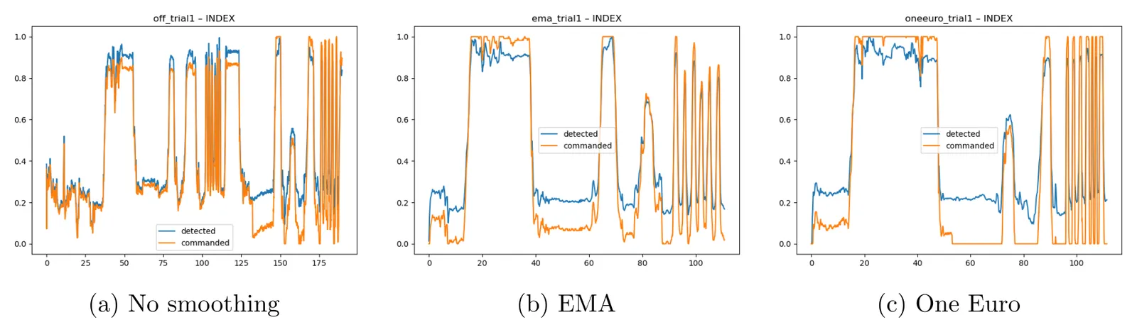
Interpretation. Unlike the thumb, the index finger exhibits consistent tracking across all smoothing methods. Differences between configurations primarily reflect the expected trade-off between responsiveness and smoothness.

Index: error distributions

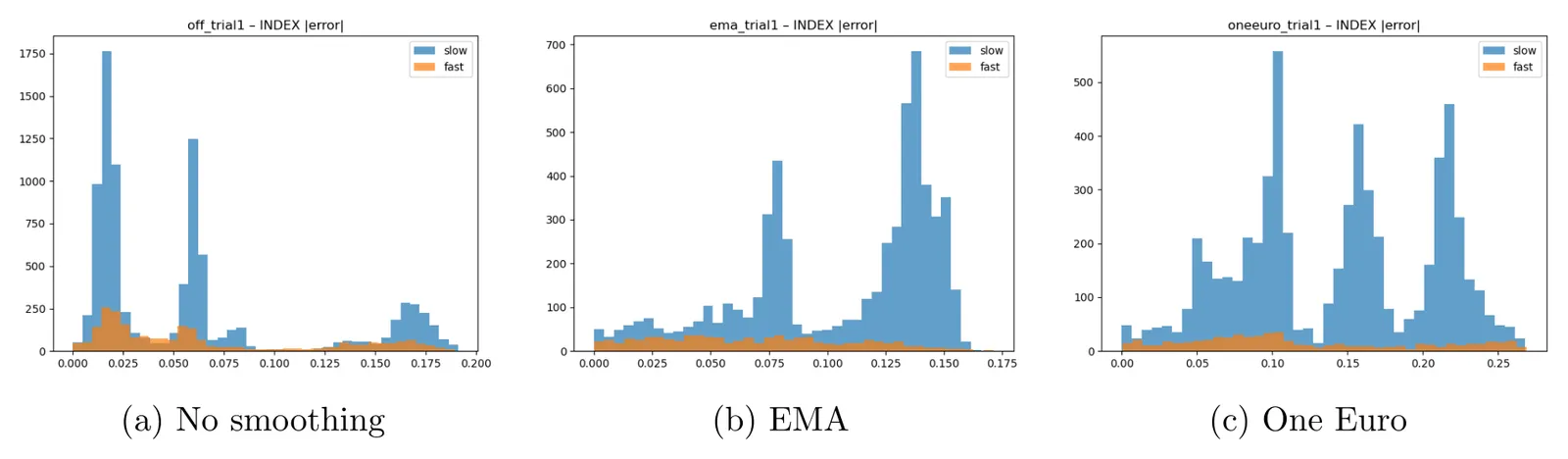
Interpretation. For the index finger, EMA achieves a good balance between reduced high-frequency noise and acceptable tracking error. No smoothing yields slightly lower RMSE but with higher temporal variability.

Discussion

The experiments reveal a clear difference between the thumb and the other fingers. For the index finger, all three smoothing methods produce usable trajectories, and the main trade-off is the expected one between responsiveness and smoothness. EMA gives the smoothest visual result, while no smoothing retains the fastest response at the cost of increased variability.

For the thumb, however, the dominant source of error appears to be geometric rather than temporal. Even when smoothing suppresses high-frequency fluctuations, the underlying signal remains unstable because the thumb angle itself is not consistently defined under changing wrist orientation and partial landmark distortion.

This distinction is important because it shows that filtering alone cannot solve a poor state representation. In other words, if the measured thumb angle is not stable in the first place, additional smoothing mainly hides the noise rather than correcting the underlying estimation problem.

Implementation Details

Table 3: Main implementation components.

Design Rationale

A geometry-based approach was chosen instead of a learned regression model for three main reasons. First, it enables real-time execution on lightweight hardware without any training stage. Second, it provides direct interpretability: each output angle can be traced back to explicit landmark geometry. Third, it allows rapid debugging of individual components.

The trade-off is that geometric methods depend strongly on the stability and semantic consistency of landmark detection. This limitation is particularly visible for the thumb, whose motion is not well captured by a single planar angle representation.

Limitations

The logged data contains post-processed angles rather than raw landmarks, preventing recomputation of alternative thumb estimators on identical inputs. Motion execution was user-driven rather than scripted, introducing variability across runs.

Conclusion

Temporal smoothing improves stability for non-thumb fingers but cannot fully resolve thumb instability. Our experiments indicate that thumb performance is primarily constrained by geometric representation rather than filtering, motivating future work on alternative thumb angle parameterizations and reference frames.

EMG-Based Gesture Recognition Pipeline

Synthetic signal generation for pipeline validation

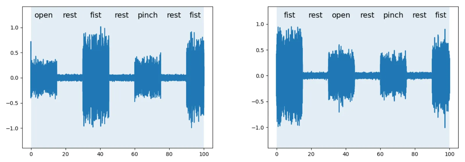
This component of the pipeline generates continuous EMG-like synthetic data. It concatenates blocks of predefined gestures with a given duration. For each gesture block, activity is synthesized by filtering Gaussian noise with a Butterworth band-pass filter, which is centered around a predefined gesture frequency — effective enough for pipeline validation. Rest segments are alternated with gesture segments to include non-active intervals. In the final signal, low-magnitude Laplace samples are also added to simulate sensor noise. The dummy data generator returns a sample-wise signal along with a corresponding set of intervals.

Configuration-driven preprocessing and schema validation

The preprocessing stage is fully configuration-driven to ensure reproducibility and experimental control. All acquisition and segmentation parameters, including sampling rate, window and hop size, gesture definitions with a fixed label mapping, and file path templates, are defined in an external YAML file. A dedicated schema layer loads this configuration with validated defaults, enforces strict consistency checks such as exact alignment between gestures and label-map keys, and derives window lengths deterministically from the sampling rate. It also provides small but critical utilities, including millisecond-to-sample conversion and path template expansion, ensuring a single source of truth across experiments while supporting both raw-signal and envelope processing modes.

Sliding-window segmentation and labeling

The passed EMG signal is segmented into overlapping sliding windows. Given sampling rate $f_s$, the function extracts windows of length $W\ \text{ms}$ — a sequence of fixed-size samples. Each window is assigned a label through a majority vote based on overlap, where labels are available: the window is assigned the label that has the largest total overlap. The segmentation outputs windowed data, window labels, and corresponding time interval boundaries, to ensure correct agreement of samples and annotations.

Recurrent Neural Networks

RNN suitability

RNN models are suitable, as hand movement is intrinsically time-dependent. Recurrent models with time-memory have the ability to recognize complex EMG temporal patterns. This is mainly due to the fact that EMG signals are sequential and non-stationary: muscle activity changes over time and gesture-to-gesture transitions can differ, which makes time-dependent memory much more advantageous. Additionally, while gestures may have similar signal at time $t$, their activation and drop-down dynamics can differ, which an RNN can recognize by leveraging the preceding context. We will be specifically using GRU/LSTM models, and later implementing bidirectional versions of the models, as gated recurrent models mitigate vanishing-gradient issues and capture both short- and long-term dependencies — supporting EMG temporal dependence as discussed previously.

Model architectures and features

Recurrent neural networks process sequential inputs $x_1, \dots, x_T$. At each timestep, the network carries forward information from the previous timestep — from internal memory, usually referred to as the hidden state. In general form, an RNN updates its hidden state at each time step, and uses the resulting hidden state to produce the output. The following equations represent the given process.

where $\phi(\cdot)$ is the activation function (e.g. $\tanh$), $o_{t+1}$ denotes output scores, and $\psi(\cdot)$ is a task-dependent activation function.

GRU/LSTM, which we will use, also include special gates that efficiently attempt to keep relevant and forget irrelevant information from the previous timestep.

Feature extraction

The current feature extraction pipeline computes three categories of statistical features from each input window and uses them as model inputs:

• Basic statistics: mean, standard deviation, minimum, maximum, range.
• Window-shape features: skewness and excess kurtosis (central moments).
• Frequency-domain features: spectral centroid, spectral bandwidth, and total spectral power.

These features may be adjusted in the next step of the research; however, they provide a solid baseline and a future reference.

GRU

The Gated Recurrent Unit is an RNN with additional gates — a reset gate and an update gate — which control how much of the previous hidden state is retained and overwritten. Given an input $x_{t+1}$ and hidden state $h_t$, the GRU additionally computes the reset gate $r_t$ and update gate $u_t$:

and a given candidate hidden state:

The new hidden state is then obtained by blending the previous state and the new candidate state:

where $\sigma(\cdot)$ denotes an activation function and $\odot$ is element-wise multiplication. The perceived gates help the model retain important information while forgetting irrelevant information from previous timesteps.

In the context of EMG signal-based gesture recognition, a key benefit of the GRU is that compared to a classic (Elman) RNN, it models temporal dependencies more effectively while adding only little complexity in both training and inference. A potential drawback, relative to an LSTM, is that the GRU is most often a smaller and simpler architecture and, therefore, may capture long-term dependencies less effectively. However, this limitation may not be crucial for gesture EMG, since the relevant dependencies may be short- to mid-range: after a few gestures, earlier context may no longer be needed.

LSTM

Long short-term memory networks are typically larger than GRUs because they extend the standard RNN structure by adding a separate cell state and three additional gates — the candidate cell state $\tilde{c}_t$, the forget gate $f_t$, the input gate $i_t$, and the output gate $o_t$ — which are computed the following way:

After computing the gates and candidate cell state, the cell state is updated and the new hidden state is then computed:

The notation is kept consistent with that in the previous GRU section.

LSTMs have a more complex structure than GRUs, which helps them better capture longer-term dependencies. In our case — EMG-signal gesture prediction — whether an LSTM architecture is worth it depends on whether the signals carry some sort of meaningful long-term dependencies, and how much these features actually matter in the prediction. On top of that, if we want independent integration of the network on a Raspberry Pi in the future, then model complexity and size become even more of a burden.

RNN pipeline validation

After running both a GRU and an LSTM network through the full pipeline on a 10,000-second synthesized sample (7 epochs, $f_s = 1000$) we yield the following performance metrics.

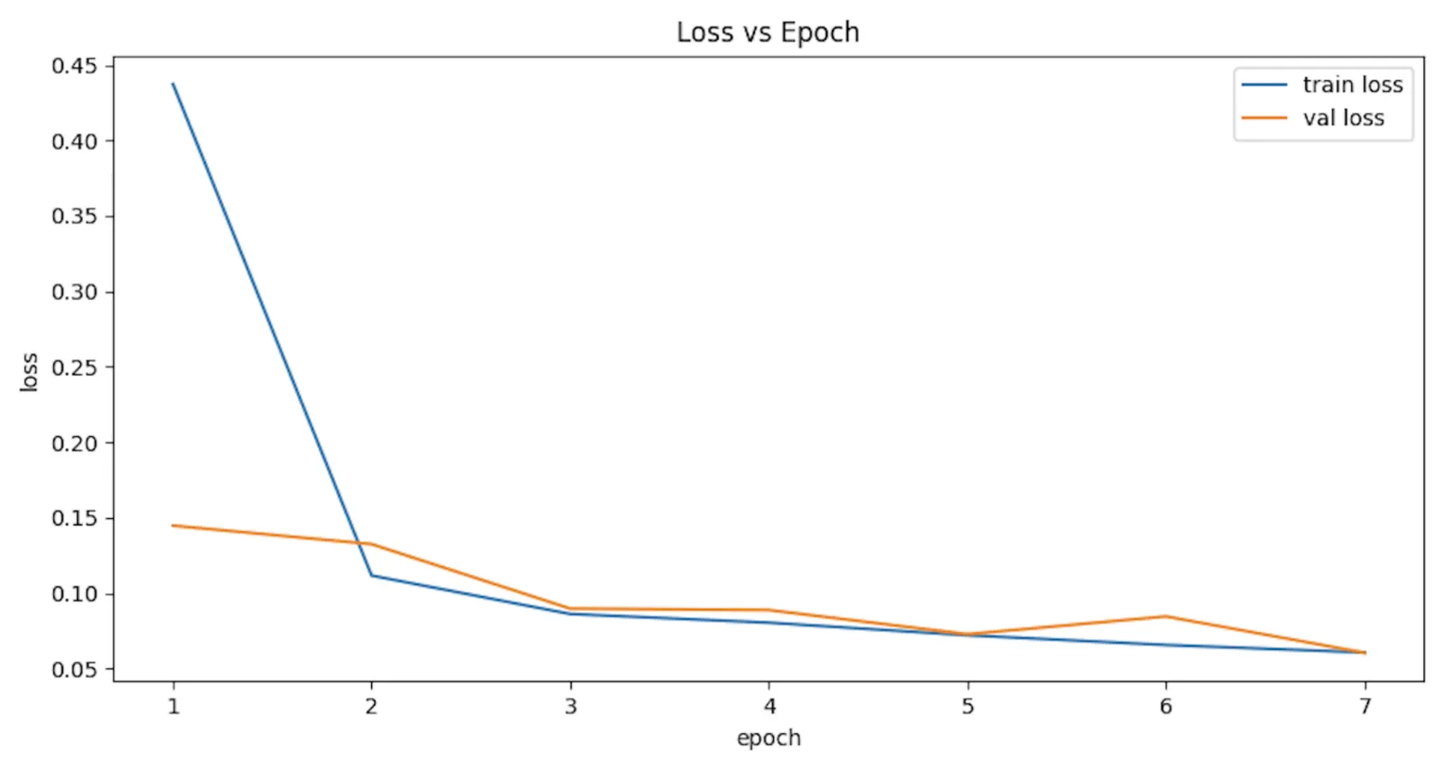
Table 4: GRU metric report (macro F1 = 0.9743, weighted F1 = 0.9798).

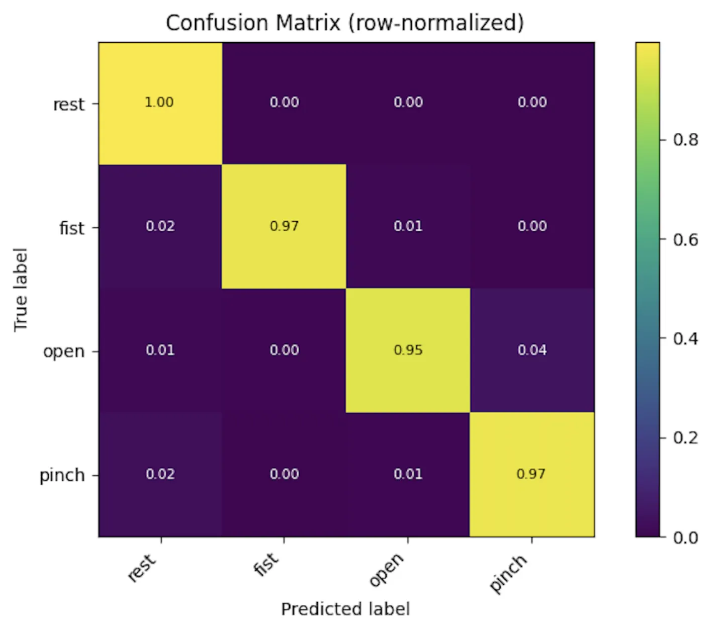
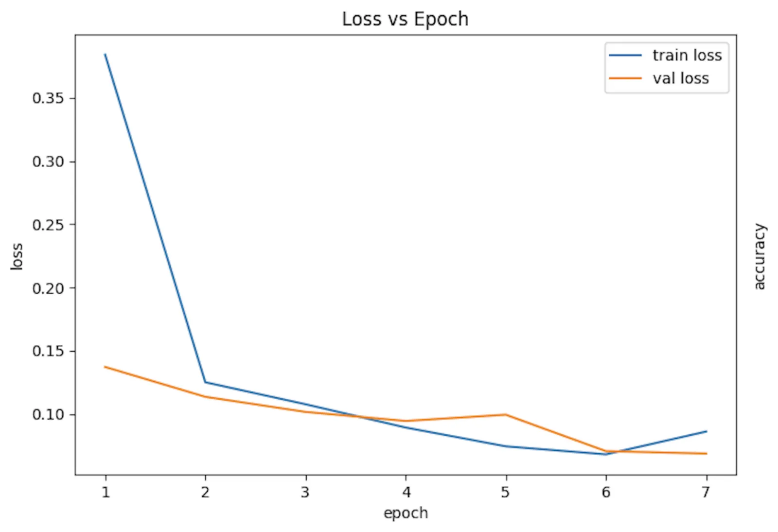
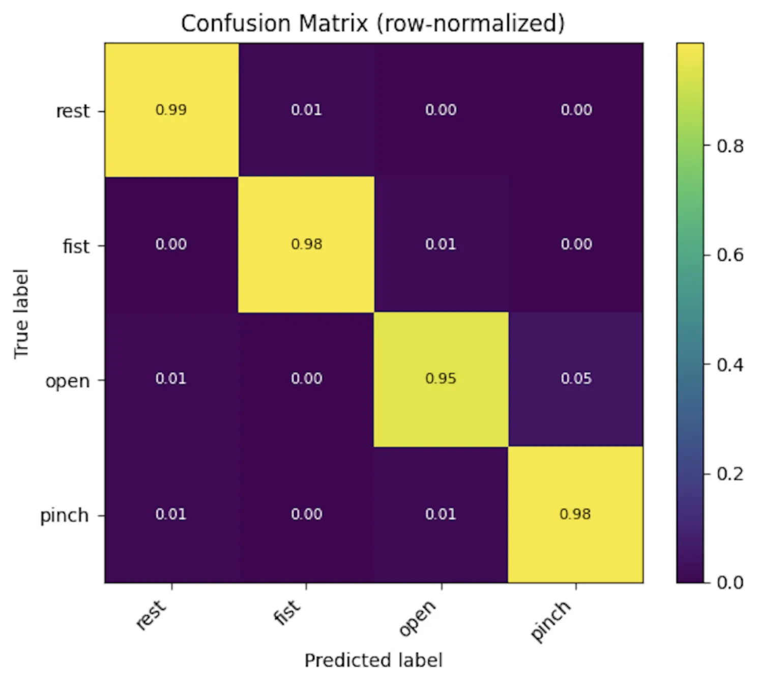
Table 5: LSTM metric report (macro F1 = 0.9704, weighted F1 = 0.9771).

While we cannot draw meaningful conclusions from these results, as they are based on synthesized data, they do confirm that the end-to-end pipeline functions correctly and is ready for further analysis when real data is collected.

Convolutional Neural Network

Suitability of the approach

Surface electromyography (sEMG) captures the spatiotemporal summation of motor unit action potentials (MUAPs) across the skin surface, serving as a non-invasive conduit to human motor intent. The accurate decoding of these stochastic, non-stationary signals constitutes the primary functional block in myoelectric control interfaces for neuroprosthetics, robotic manipulators, and extended reality (XR) hardware [1].

Historically, sEMG classification relied heavily on classical machine learning topologies, most notably the Support Vector Machine (SVM) and Random Forest classifiers. While SVMs excel in high-dimensional margin separation, they depend fundamentally on the manual extraction of heuristic time-domain (e.g. Mean Absolute Value, Zero Crossings) and frequency-domain (e.g. Median Frequency) descriptors [2]. This reliance on handcrafted feature engineering inherently constrains the model’s capacity to uncover latent, nonlinear relationships within the raw myoelectric signal. To address the temporal dynamics of sEMG, subsequent literature explored Recurrent Neural Networks (RNNs) and Long Short-Term Memory (LSTM) architectures. While LSTMs natively ingest sequential data and accommodate long-term dependencies, they suffer from high computational complexity, challenging sequential training dynamics, and latency overheads that hinder real-time micro-controller deployment [3].

Objective

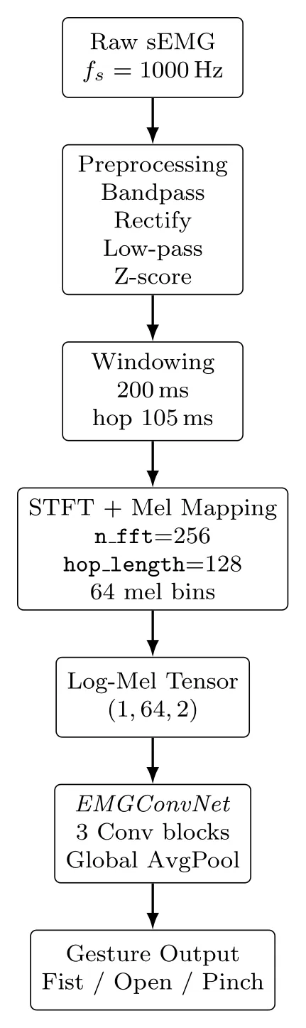
This section proposes an alternative topological framework: transforming the temporal sEMG signal into a 2D pseudo-image via short-time Fourier transform (STFT) log-mel spectrograms, and applying a highly constrained, lightweight Convolutional Neural Network (CNN). Unlike SVMs, CNNs implicitly perform hierarchical feature extraction directly from the time-frequency topography. Unlike RNNs, CNNs parallelize computation over the spatial grid, jointly capturing spectral density and temporal morphology without the recursive latency bottleneck [4].

The pipeline is grounded in an accompanying software implementation that fully specifies preprocessing, windowing, spectrogram generation, model architecture, training, and evaluation. Our contribution is a fully specified, reproducible, end-to-end pipeline tailored for extreme short-window low-latency interfaces, culminating in a custom CNN architecture designed to avoid dimensional collapse on microscopic spectrograms.

Methodological paradigm and architecture comparisons

Table 6: Methodological comparison of short-window sEMG classification paradigms.

The limitation of classical classifiers (SVMs). Classical approaches isolate spatial representations through predefined mathematical descriptors. While computationally cheap during inference, standard SVM pipelines are statistically brittle when presented with muscle fatigue, electrode shift, and inter-user anatomical variability [2]. The assumption that a discrete set of engineered features comprehensively spans the informative variance of an sEMG window is fundamentally restrictive. The proposed CNN approach circumvents this by treating the STFT-generated matrix as a continuous sensory field, enabling the optimization algorithm (Adam) to natively sculpt Gabor-like filter banks tailored strictly to the discriminative task, substantially elevating the representational ceiling over SVM baselines.

The case against pure recurrence (RNNs/LSTMs). sEMG signals are temporal sequences, naturally suggesting the application of RNNs. However, the stochastic firing rate of motor units (typically 10 Hz to 20 Hz) combined with typical sampling rates (1 kHz) creates sequences of thousands of discrete datapoints per gesture [3]. RNNs operating on raw 1D sequences struggle to compress redundant spectral information efficiently. Even when LSTMs are fed windowed features, backpropagation through time (BPTT) is computationally expensive and memory-intensive. In contrast, transforming each window into a spectrogram compresses the temporal dimension algorithmically (via STFT overlap) and expands the spectral dimension, allowing 2D convolutional kernels to concurrently inspect time and frequency without sequential state maintenance.

Data conditioning pipeline

Continuous 1D sEMG streams sampled at $f_s = 1000\ \text{Hz}$ undergo a rigorous preprocessing pipeline to suppress artifactual noise while preserving the envelope of MUAP bursts.

1. Bandpass filtering: a 4th-order Butterworth bandpass filter with cutoff frequencies corresponding to 20 Hz to 450 Hz is instantiated. This eliminates low-frequency cable sway and galvanic skin drift while obeying the Nyquist criteria to avoid aliasing 60 Hz/50 Hz mains harmonics.
2. Full-wave rectification: the bipolar signal is transposed into a unipolar magnitude space via absolute value operations, translating the alternating current-like signal into a power-equivalent geometry.
3. Low-pass smoothing: a 10 Hz low-pass Butterworth filter generates the linear envelope of the signal, functioning as an analog integration of the motor unit recruitment density.
4. Z-score normalization: the amplitude is dynamically standardized to zero mean and unit variance ($\mu = 0,\ \sigma = 1$) to stabilize initial gradient descents and counteract signal attenuation due to variable skin impedance.

STFT and log-mel spectrogram derivation

For low-latency control algorithms, the allowable system delay is strictly bounded. We implement a sliding window constraint of 200 ms (200 samples) with a 105 ms hop length.

To transition to the visual domain, we employ the Short-Time Fourier Transform (STFT):

Specifically, we dictate a Hann window weighting $w(n)$ with parameters $\texttt{n\_fft} = 256$ and $\texttt{hop\_length} = 128$. The corresponding power spectrogram $P = |X|^{2}$ highlights the spectral energy distribution.

To compress the frequency bands in a manner that isolates the fundamental frequencies of muscle activation, we project the linear frequencies onto $n_{\text{mels}} = 64$ mel filterbanks bounded between 20 Hz and the 500 Hz Nyquist limit. Finally, to handle the vast dynamic scale of muscle activation (ranging from baseline noise to maximal voluntary contraction), we apply specific logarithmic compression:

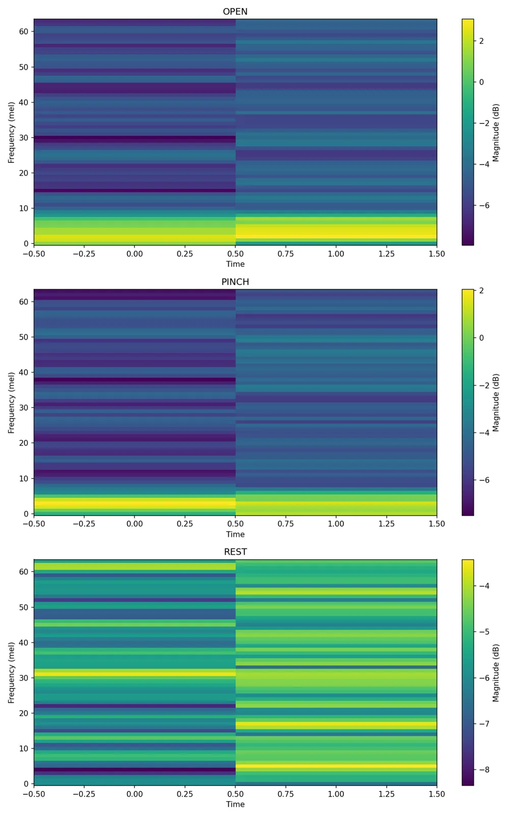
This bounds matrix values, improving neural numerical stability. Crucially, a 200 ms window parsed through an STFT of $N = 256$ and hop of 128 yields an exceptionally small tensor: $64 \times 2$ (frequency $\times$ time).

Network topology: EMGConvNet

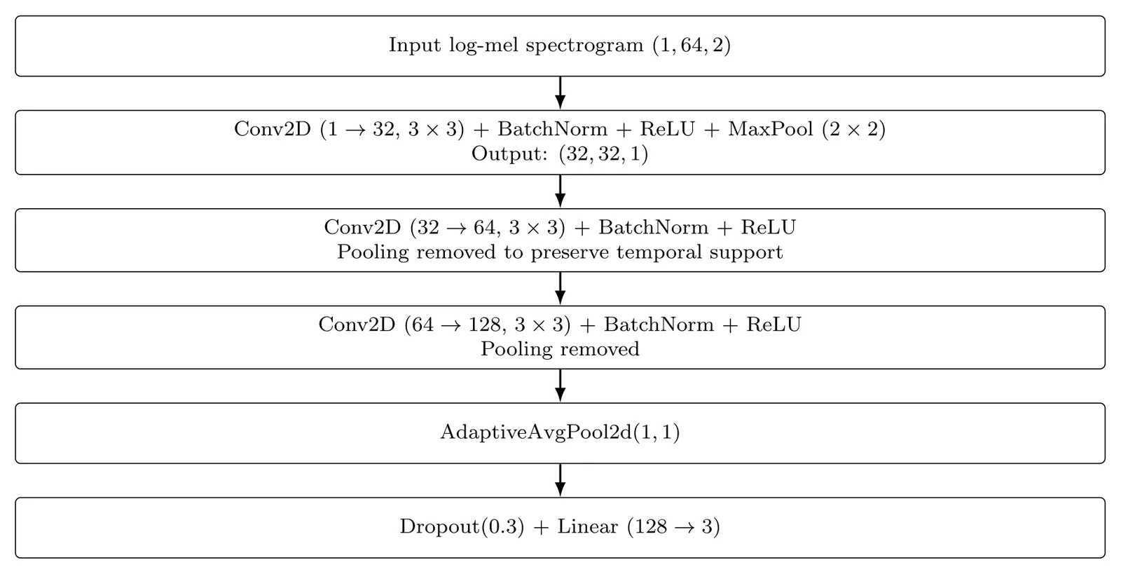
The diminutive nature of the $(1, 64, 2)$ input matrix necessitates a paradigm deviation from standard VGG-like or ResNet architectures. If temporal downsampling (via $2 \times 2$ max pooling) is applied repeatedly, the 2-frame time dimension immediately collapses to zero, obliterating the forward pass matrix computations.

We construct EMGConvNet, a compact spatial hierarchy specifically engineered for short-time-frame time-frequency arrays:

• Block 1 (stem): $\text{Conv2D}(1 \to 32, 3 \times 3) \to \text{BatchNorm2d} \to \text{ReLU} \to \text{MaxPool2d}(2 \times 2)$. The input $(1, 64, 2)$ becomes $(32, 32, 1)$.
• Block 2: $\text{Conv2D}(32 \to 64, 3 \times 3) \to \text{BatchNorm2d} \to \text{ReLU}$. Pooling is explicitly removed to protect the dimension scalar.
• Block 3: $\text{Conv2D}(64 \to 128, 3 \times 3) \to \text{BatchNorm2d} \to \text{ReLU}$. Pooling is explicitly removed.
• Global feature aggregation: $\text{AdaptiveAvgPool2d}(1, 1)$. This enforces strict translation invariance and collapses the remaining tensor explicitly into a flat 128-dimensional embedding vector.
• Linear classifier: $\text{Dropout}(0.3)$ for mitigating dataset overfitting, followed by a dense projection to $K$ classes ($128 \to 3$).

The parameter ceiling is forcibly maintained at 93,283 trainable weights (an estimated memory footprint of 0.36 MB). This ensures extreme convergence velocity, zero reliance on GPU acceleration during deployment, and instantaneous sub-millisecond classification latency on generic x86 or ARM CPUs.

Baseline validation and results

To validate the programmatic integrity, gradient flow, and representational capacity of the complete pipeline, an empirical trial was executed utilizing a 60-second synthetic sEMG protocol partitioned into three gestural classes (fist, open, pinch).

The network was optimized using standard categorical cross-entropy without explicit class weighting, via Adam ($\text{lr} = 0.001$) over batches of size 32.

Strikingly, given the constrained capacity and absence of recurrent topology, the network exhibited rapid loss stabilization. By epoch 5 (total training time ~4.2 s on CPU), the system recorded a best validation accuracy of 81.58% (finalizing at 78.07%), with a macro F1-score of 0.56 mapping across 114 out-of-sample frames.

While synthetic validation does not strictly equate to inter-subject clinical generalization, it solidly corroborates the hypothesized capabilities of the CNN to learn discriminative manifolds from severely restricted temporal dimensions. The results categorically validate the decision to eschew the mechanical difficulties of sequential RNN processing and the inflexibility of SVM heuristic filtering.

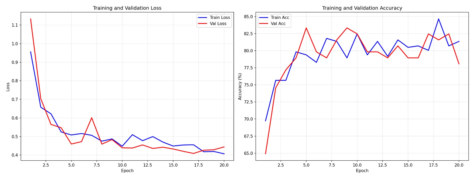
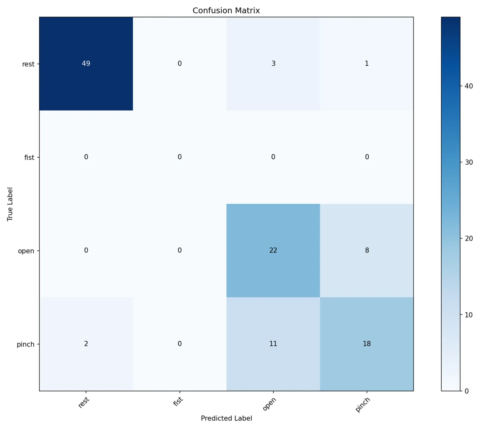
Table 7: CNN baseline evaluation report.

Discussion and future directions

The transition from generalized sequential modelling (RNN/LSTM) to spatial spectro-temporal modelling (CNN) offers a robust, highly parallelizable path forward for embedded electromyographic pattern recognition. The visual representation of the EMG signal within the log-mel envelope contains distinct spectral gradients that effectively characterize distinct physiological motor recruitments.

By actively protecting the temporal dimension through delayed max-pooling, EMGConvNet retains the temporal variation necessary for gesture transients without incurring the overhead of BPTT. Future work will entail transitioning this validated mathematical architecture to physical multi-channel sEMG arrays collecting high-density data on active human subjects, further exploring the network’s resilience to electrode displacement protocols and muscle fatigue spectrum shifts.

Statistical Analysis: Classic ML Baseline

Experimental setup

We validated the classic ML pipeline on 1000 s of synthetic EMG generated with alternating 5 s gesture blocks and rest blocks at 1 kHz sampling. Signals were segmented into 200 ms windows with a 100 ms hop (10 Hz update rate). For each window, we extracted a combined time+frequency feature set (e.g. RMS/MAV/WL/ZC/SSC/WAMP, Hjorth parameters, AR(4), Welch-PSD band powers, spectral entropy), followed by standardization. The dataset was split into train/test with an 80/20 stratified split. We report accuracy and macro-F1 (class-balanced).

Model comparison

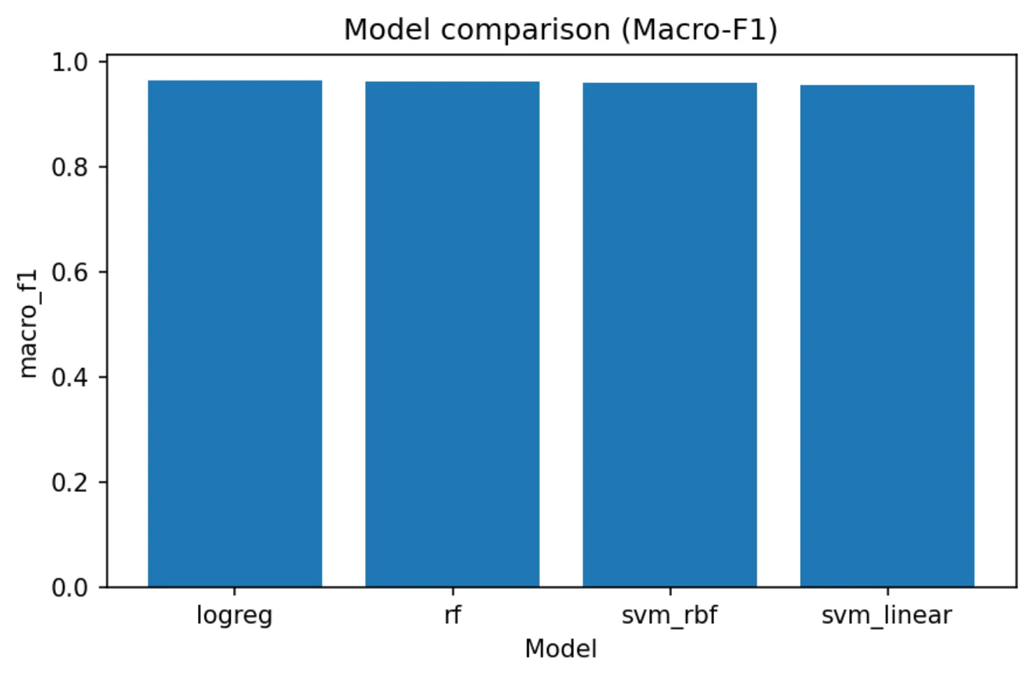
We evaluated four standard classifiers: logistic regression (L2), linear SVM, RBF SVM, and random forest.

Table 8: Hold-out test performance on 1000 s dummy EMG.

Error analysis (class-wise)

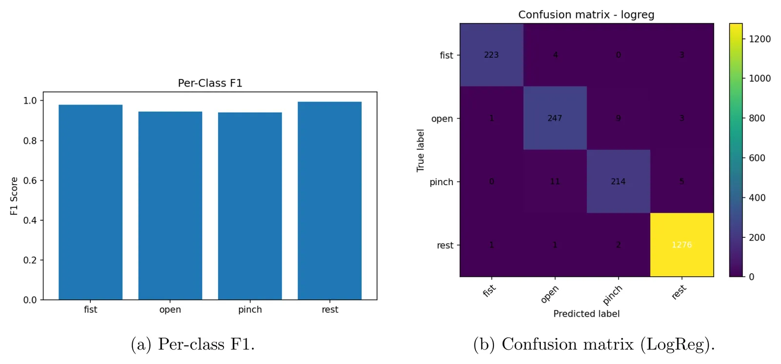
Logistic regression achieved the best macro-F1 (0.965), so we use it for class-wise analysis. The main confusion is between open and pinch, while rest is nearly perfectly separated.

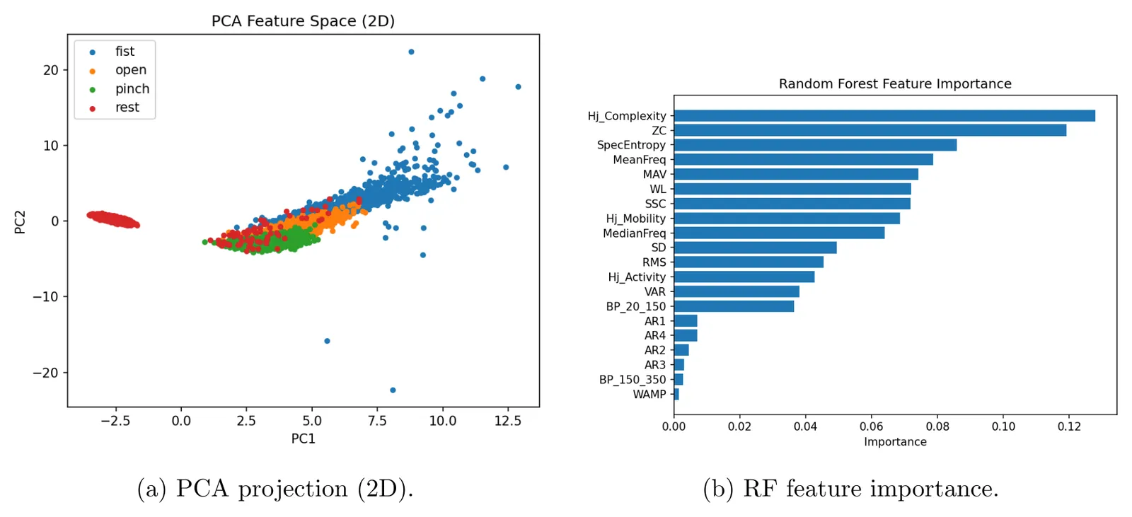
Feature space and feature importance

To understand separability, we projected feature vectors to 2D using PCA. We also inspected random forest feature importances to identify which statistics contributed most to discrimination.

Regularization study

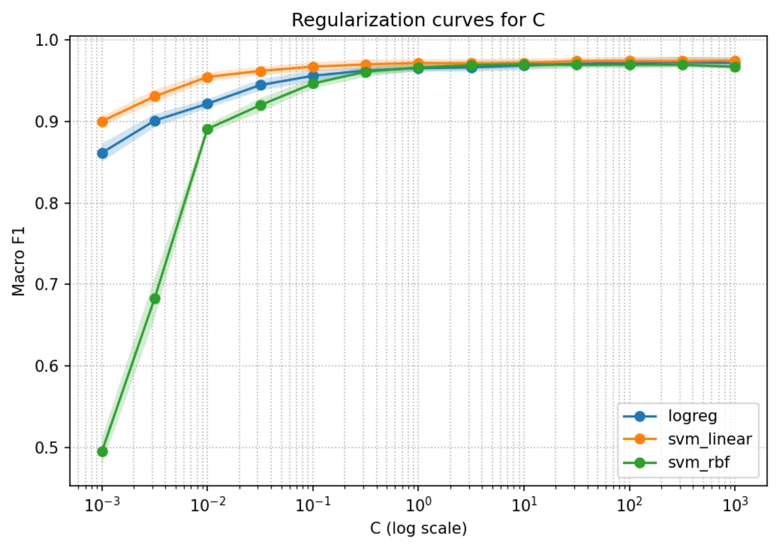
We swept the regularization parameter $C$ for logistic regression and SVMs using stratified 5-fold cross-validation and plotted macro-F1 versus $C$ (log scale) to identify stable operating regions.

Limitations and scope

These results validate the pipeline on controlled synthetic EMG and mainly serve as a statistical baseline and interpretability reference. Real-time performance on hardware is expected to be lower due to nonstationarity (electrode shift, muscle fatigue, subject variation) and additional constraints (latency, drift), so future work will focus on evaluation on real recordings and robustness across sessions and subjects.